


The most renowned optical designs achieved fame by combining multiple elements into a single system. Multiple elements minimize aberrations, because each lens (at least partially) cancels aberrations introduced by the others. The nearly arbitrary surface figure of modern aspheric lenses condenses aberration correction into fewer elements, allowing significant volume and weight reductions. But the full potential of aspheric lenses is only reached when design, fabrication and end application parameters all align, and that starts with proper specification.
Properly specifying your optics is nothing new, but the particulars of asphere fabrication introduce extra complexity. Specifically, aspheres are fabricated with subaperture tools. This means deviations from the design surface figure can occur at a range of spatial frequencies. A spherical lens might be prone to, say, a slowly increasing error from the edge towards the center. Those errors are at a low spatial frequency — essentially at a scale of the full diameter of the optic. Because aspheric tools are significantly smaller than the full optic, it is possible to have deviations at mid-spatial frequencies — essentially at the scale of the size of the tool.
The problem is that the same peak-to-valley (PV) deviation affects system performance differently if surface errors are at different spatial frequencies. Even putting a tolerance on the allowable slope error cannot eliminate the issue, as it only looks at a bandwidth, defined by the window size used for the measurement. This is not just an academic exercise; the spatial frequency of surface irregularities directly impacts the performance of aspheric lenses. Understanding these effects will allow for the proper specification of aspheric lenses to meet your application requirements. A useful metric for analyzing the performance of an asphere is the Strehl ratio.
Measuring image quality
A number of metrics quantify image quality; the Strehl ratio is noteworthy for being both powerful and simple to calculate. The Strehl ratio is the ratio between the peak irradiance of a focal spot compared to the (theoretical) peak irradiance of an aberration-free system. For systems close to diffraction-limited, it is an excellent indicator of system performance.
In fact, “diffraction-limited” is often defined as a Strehl ratio greater than 0.8. In that regime, the Strehl ratio can be approximated by,
where ![]()


is the RMS surface error in waves. Obviously, the Strehl ratio decreases with increasing surface irregularity, but less obvious is the fact that it also decreases with an increasing number of cyclic variations, or increasing spatial frequency. That is, a 50mm diameter lens with five periods of cyclic error at a spatial frequency of (10mm)-1 will have a higher Strehl ratio than the same lens with twelve-and-a-half periods of cyclic error of the same magnitude with a frequency of (4mm)-1.
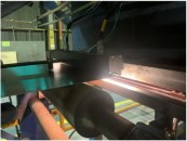
How does the Strehl ratio help evaluate optical system performance? Consider, for example, a laser etching system. The etching rate depends upon the power density delivered to the target material. The Strehl ratio is essentially a measure of how much of the theoretical maximum power density is being delivered. In this case, the Strehl ratio is a direct measurement of the actual system performance. For imaging systems, the situation is a little more complex, but here you can think of the Strehl ratio as an indication of how much the image of a point source spreads out. The lower the Strehl ratio, the more a point source will be “spread out” and the more the image will be blurred. The Strehl ratio does not provide the detailed performance prediction you can get with the modulation transfer function (MTF), but it will generally be true that a lower Strehl ratio corresponds to a lower quality image.
Spatial frequency and Strehl
Surface irregularities — that is, deviations from a surface’s nominal shape — can be split up into three groups: low, high, and mid-spatial frequency errors. Low spatial frequency errors are those that generally result from the use of full aperture (or larger than full aperture) tools. High spatial frequency errors are typically classified as surface roughness and generally cause high-angle scattering. The final category, mid-spatial frequency errors, is a particularly troublesome category of surface irregularities.
Mid-spatial frequency errors are troublesome because, as shown in Figure 1, the exact same PV error will degrade the Strehl Ratio differently depending upon the frequency. Qualitatively, you can understand this effect by referring back to geometric optics. The deviation of a light ray is approximately proportional to the angle it makes with respect to the normal of a surface. If the surface deviates from the desired profile by, say, 0.1µm over a distance of 10mm, then the angle of incidence will be different by approximately 10µrad (microradians) from the design value. The same 0.1µm deviation over only 1mm, however, will change the angle of incidence from the design value by approximately 100µrad — 10X greater variation from the same PV error.
That qualitative discussion hints at how proper specification can ameliorate the potential issues associated with asphere fabrication.

Figure 1: For a given PV surface irregularity the Strehl ratio is lower for higher spatial frequencies in the mid-frequency range.
Getting the most from your asphere
The greater ray deviation at higher spatial frequencies occurs because the surface is “steeper” for a given PV variation. That is, as shown in Figure 2, the slope of the error is higher at higher spatial frequencies. Placing a specification on the slope error will catch those mid-spatial frequency errors.

Figure 2: The surface deviation as a function of position shown on the right has a much steeper slope than the function on the right with a lower spatial frequency. Placing a specification on the slope error will exclude optics that degrade image quality too much.
You can catch the same errors by specifying the power spectral density of the surface irregularity. You can then constrain both the total surface irregularity and the irregularities within a given spatial frequency range. This will catch the same deviations as the slope error specification while providing more detailed information about the error distribution.
Refinements of those two basic specifications offer additional control over the acceptable surface figure. For example, the errors can be divided into radial and tangential components, giving insight into the manufacturing process and providing a convenient way to investigate their effect on system performance.
You can also specify different slope errors for different regions of the lens. For example, compliant tools often are subject to roll-off error near the edge of an optic, but the system design can compensate for this, so you can loosen the tolerance for slope error at the edge. That can help control costs by avoiding unnecessarily stringent specifications. This cannot be done as easily by specifying power spectral density.
When incorporating aspheres into an optical system, it is essential for system designers to find a fabricator who can help you understand the implications of the specifications on cost and performance. The goal, of course, is to specify your components tightly enough to do the job, but not so tightly that you introduce unnecessary costs. The unique features of asphere fabrication require special attention, but a competent component supplier will partner with you to maximize the performance of your system.
Written by Wilhelmus Messelink, Technology Manager and Cory Boone, Lead Technical Marketing Engineer, Edmund Optics